how-to-feature-to-model

Input - the marts, and one question asked of every single column

This skill reads the marts produced by how-to-schema-and-warehouse. They are clean. Clean is not the same as modellable. Before a single feature is written, every column gets the same question: could a scorer have read this at the moment it had to decide? Three columns fail that question, and each one fails differently.

Population: 39,046 delivered orders carrying 2,672 returns, a base rate of 6.84%. A cancelled order cannot be returned, which is exactly why status is so dangerous as a feature.

Sample data - the same seeded marts, and what makes them a modelling minefield

No new generator: the marts already exist (seed 42). Four quirks were planted in them long before this skill, and each one attacks a model at a different seam.

Objective - which orders get held, not "predict returns"

Everrest runs a pre-dispatch QC hold: repack and photo verification on orders it believes will come back. The hold costs money and delays the order, so it can only be spent on a minority. A model that ranks well but cannot name the orders to hold has not finished the job.

Find-skills - four small modules that do the unglamorous half

The modelling library is off the shelf. What was missing was everything around it, so this skill ships it: four dependency-light modules (numpy and pandas only), each usable on its own against your own table without running the rest of the pipeline.

Build - six pipelines, one ceiling, and a decision in dollars

One deterministic script (seed 42, two runs byte-identical) walks from the marts to a signable policy. Grab the real code:

5a · Ask when each fact becomes knowable, not just what it says

This is the step almost every tutorial skips. That an order happened is known instantly. Whether it came back is known up to 20 days later. Using one as-of cutoff for both quietly trains the model on labels that had not been observed.

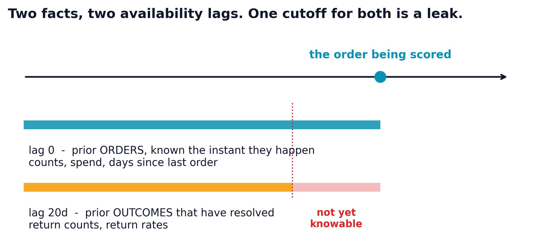
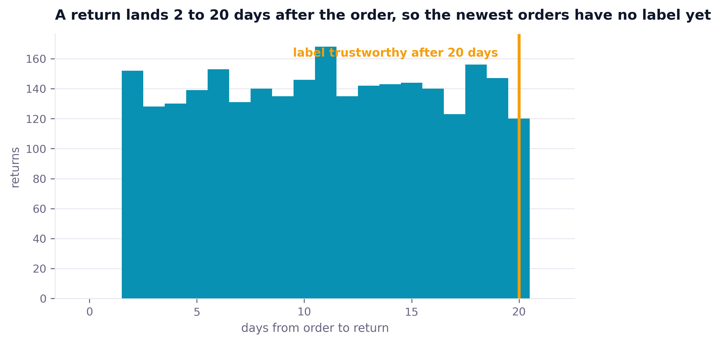
The maturity window is measured, not chosen: 20 days covers 99% of observed return arrivals.

5b · Cut the label where the clock has not finished

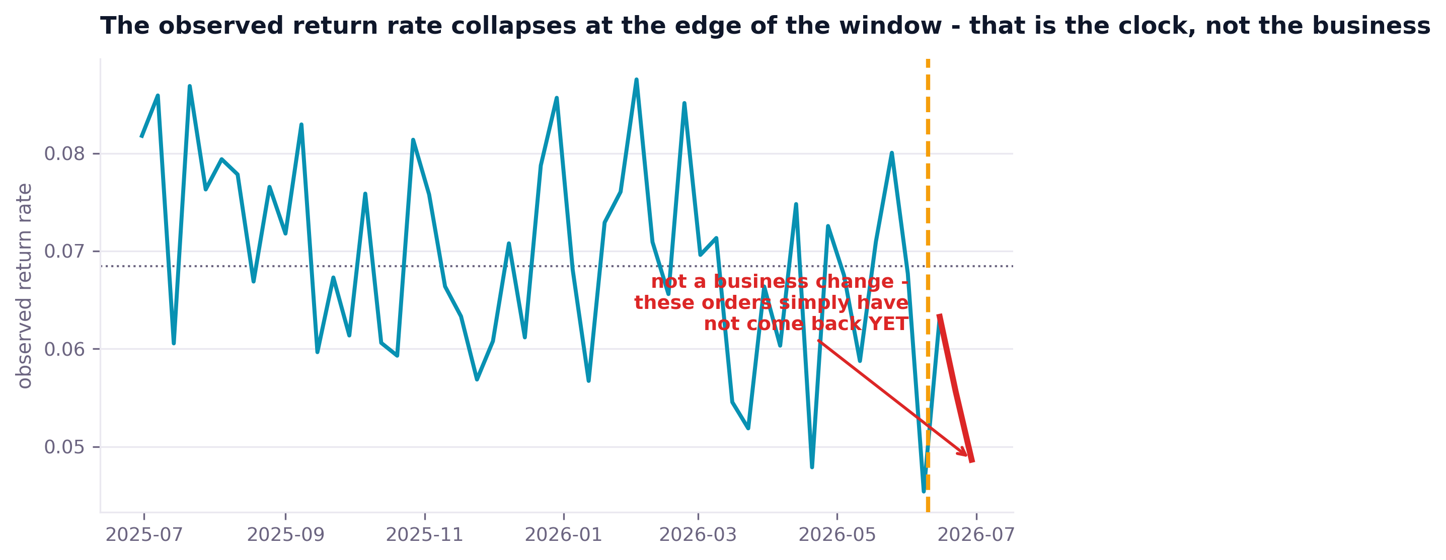
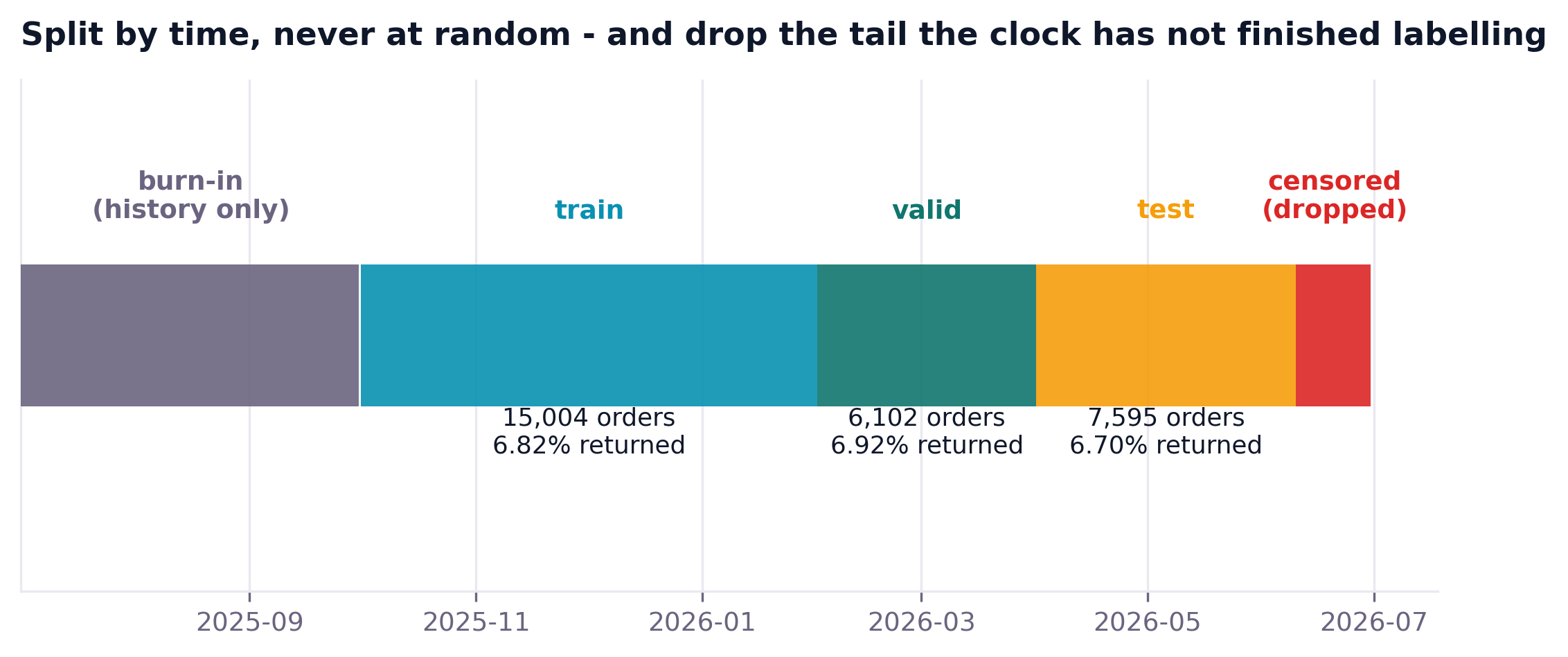
Left: the return rate appears to collapse at the edge of the window. That is the calendar, not the business - those orders simply have not come back yet. Their apparent rate is 5.18% against a true base of 6.84%. Right: so 2,334 rows after 2026-06-10 are dropped rather than labelled zero, and the split runs by time with a burn-in that exists only to build history.

5c · The leak ladder - and the number that makes it provable

Because the generator draws returns from merchant tier alone, the Bayes-optimal AUC can be computed. On a finite test set even the perfect scorer returns a random number, so it is a band, not a line. Each rung is judged against the ceiling for its own population.

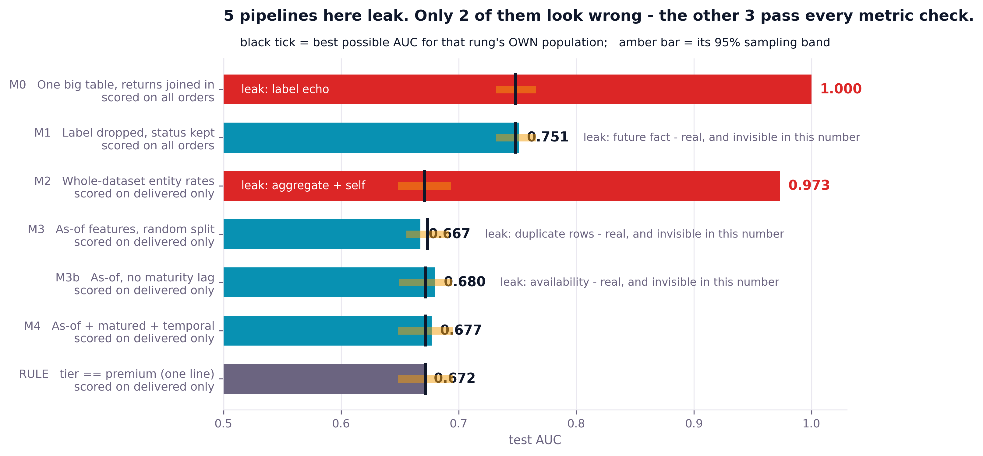
That is the finding worth carrying to your own work. A held-out score is not a leak detector - it exposes a leak only when the leak happens to be enormous. Catching the rest means reading the pipeline.

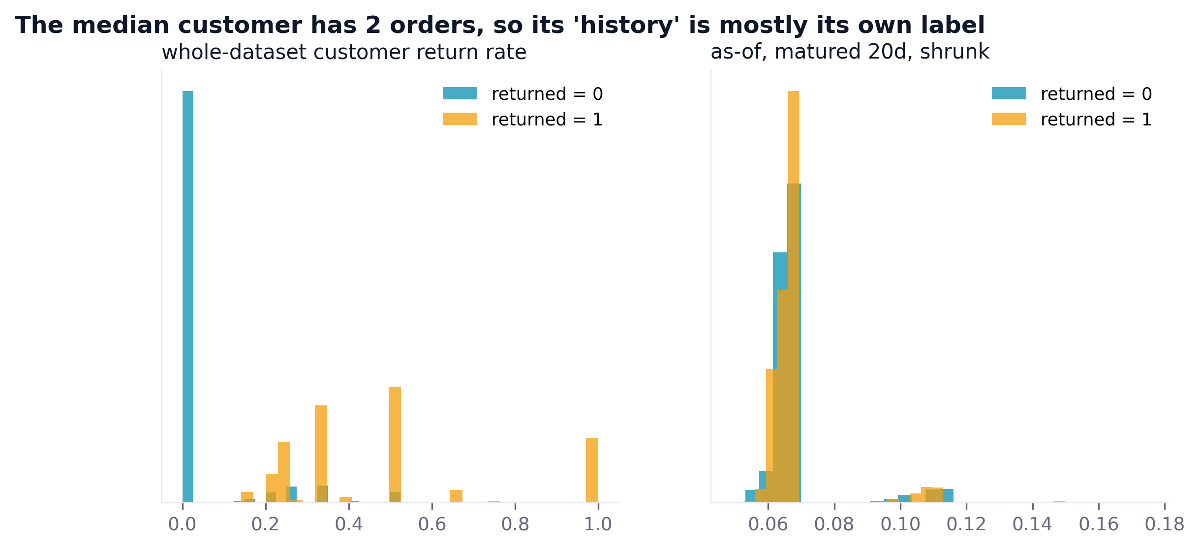
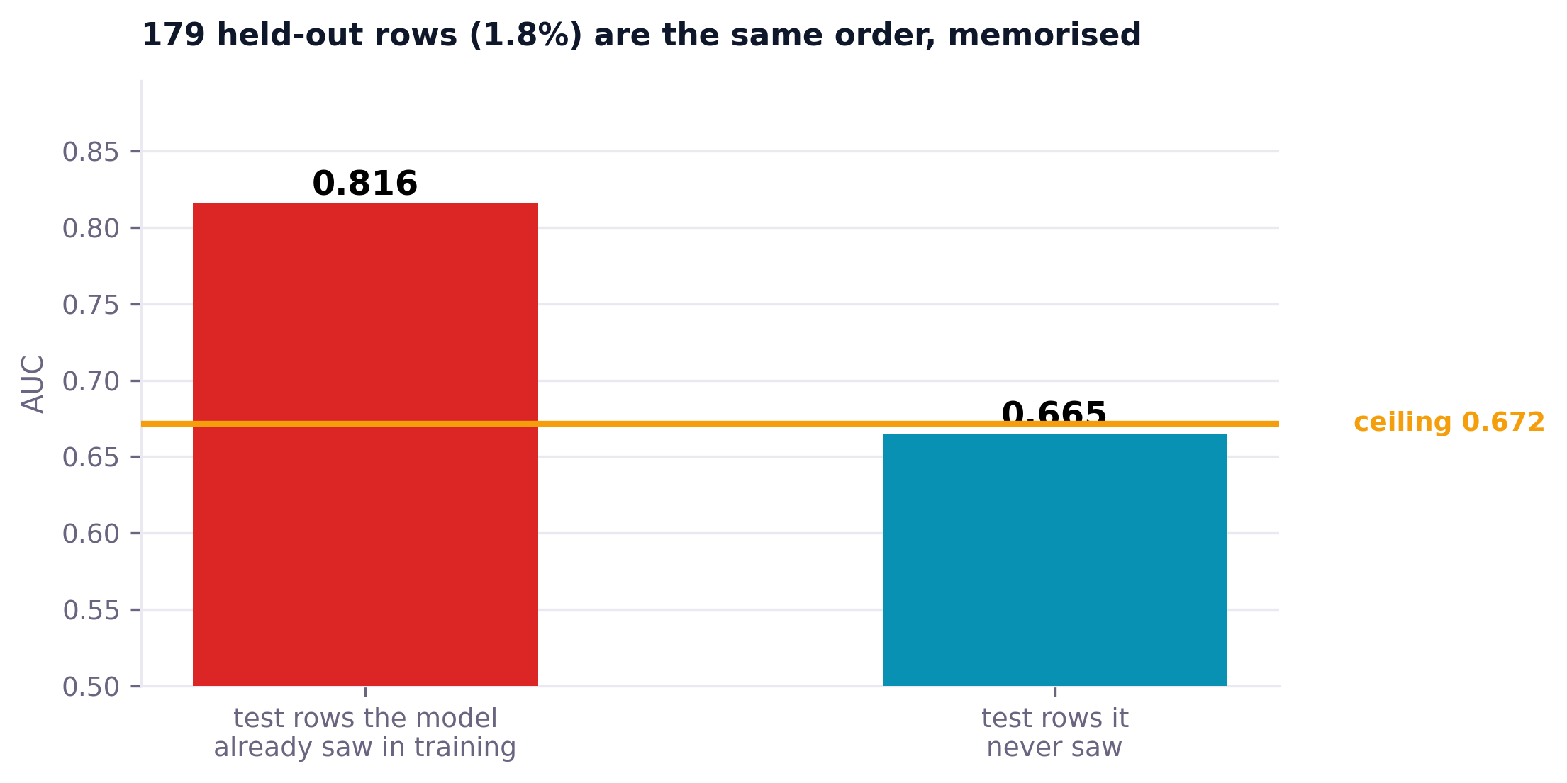
Left: the median customer has 2 delivered orders, so a groupby.transform("mean") "history" is substantially the row's own label handed back to it. Right: the duplicate leak is severe where it lands - 0.816 on the 179 memorisable rows against 0.665 elsewhere - and completely invisible in the headline, because those rows are 1.8% of the test set. At a 20% duplicate rate, one bad backfill, it moves the headline and you ship it.

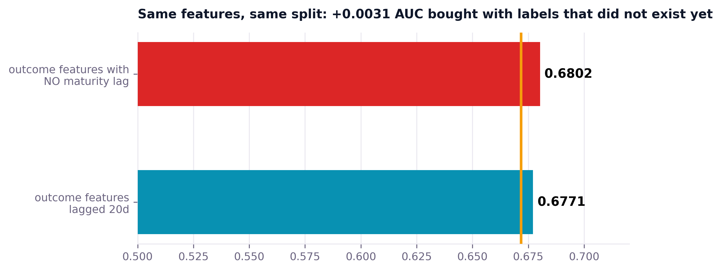
The availability leak is worth only +0.0031 AUC here, well inside the band. Undetectable, and still wrong: in production those features would be computed from a warehouse that has not received the returns yet, so the model would meet inputs it never trained on.

5d · The screen that reads the pipeline instead of the score

Because three of the five leaks are invisible in the metric, the check has to look at the table. This is a real captured run of leakcheck.audit() against the naive one-big-table version - 8 findings, 4 critical:

[!!] ceiling_breach     -
     measured AUC 0.9732 exceeds the defensible ceiling 0.6717 by +0.3015.
     Something in the table knows the answer.
[!!] random_split       order_ts
     100.0% of training rows are NEWER than the oldest held-out row.
     The model is being asked to predict the past.
[!!] label_echo         cust_rate_global
     alone scores AUC 0.9632. A single column this good is almost always
     the answer written down somewhere.
[!!] missingness_echo   return_lag_days
     is null for 94.7% of rows and the NULLNESS alone scores AUC 0.0000.
     The join that created this column probably only fires after the outcome.
[! ] constant_subset    status
     level 'cancelled' covers 3,997 rows and the label is always 0 there.
     If that is knowable only after the decision, it is a future fact.

It is a screen, not a proof. It cannot know which of your columns is populated after the decision - only you know that. What it can do is refuse to let an obvious one through unremarked.

5e · Does the model beat one line of SQL?

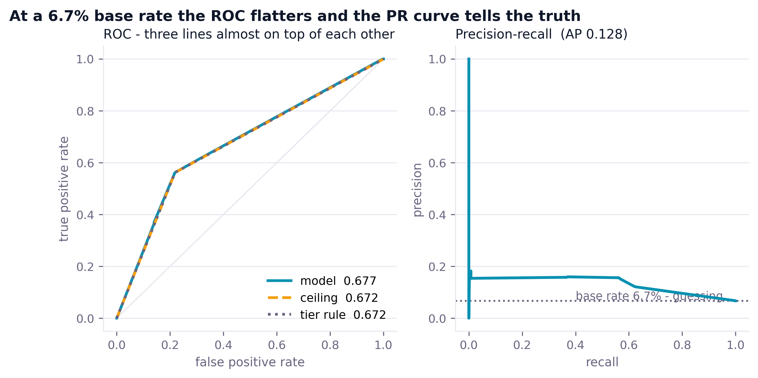
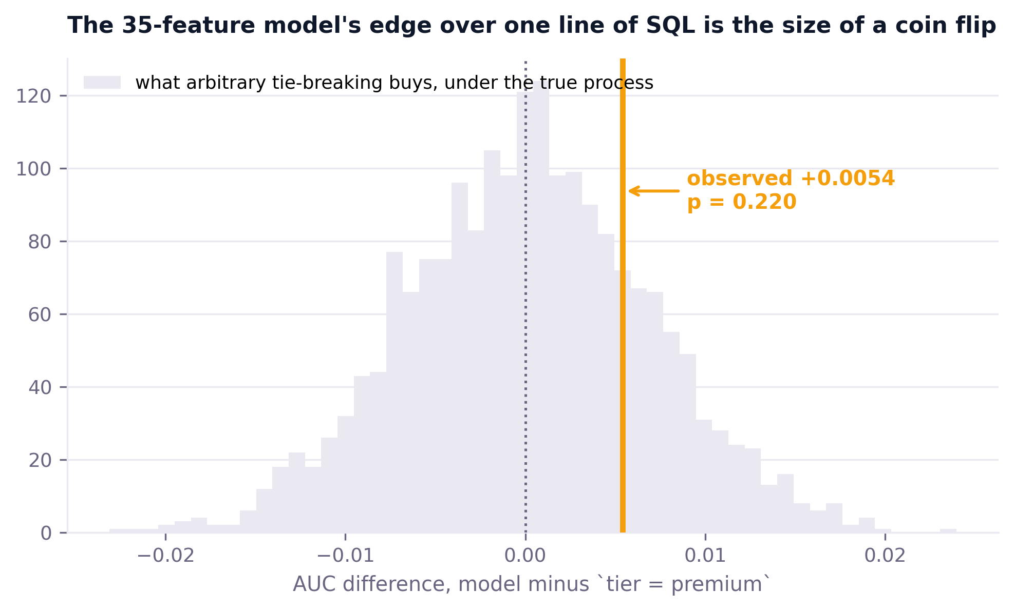
Left: three lines almost exactly on top of each other. Right: the model is +0.0054 AUC over tier = 'premium', and the correct null - redraw labels from the true probabilities, since ordering within a tier cannot carry information - puts that at p = 0.22. Note which test you run: the paired bootstrap most teams reach for gives a far tighter interval, because resampling one test set measures how stable the difference is within that sample, never whether the sample was lucky.

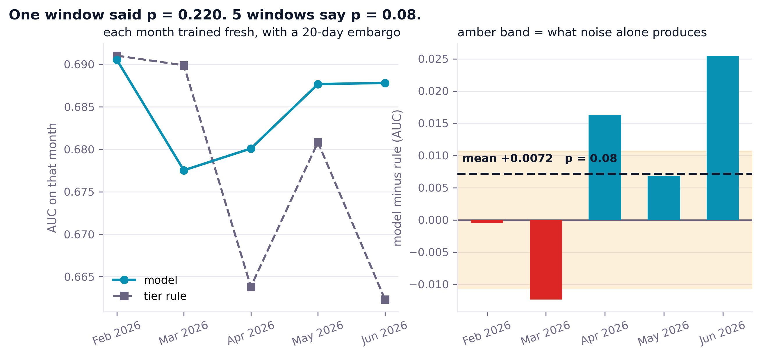
Five rolling windows, each trained fresh behind a 20-day embargo: mean +0.0072, 3 of 5 favouring the model, p = 0.08. Two windows disagree outright and the fold-to-fold spread is several times the effect. And here is the part worth keeping: we KNOW the true difference is exactly zero, and the evidence still lands at p = 0.08 - the kind of number that gets a model shipped in a Friday review. A p-value near 0.1 on a true null is not a rare accident. It is what a true null produces about one time in ten.

5f · What 35 features actually bought

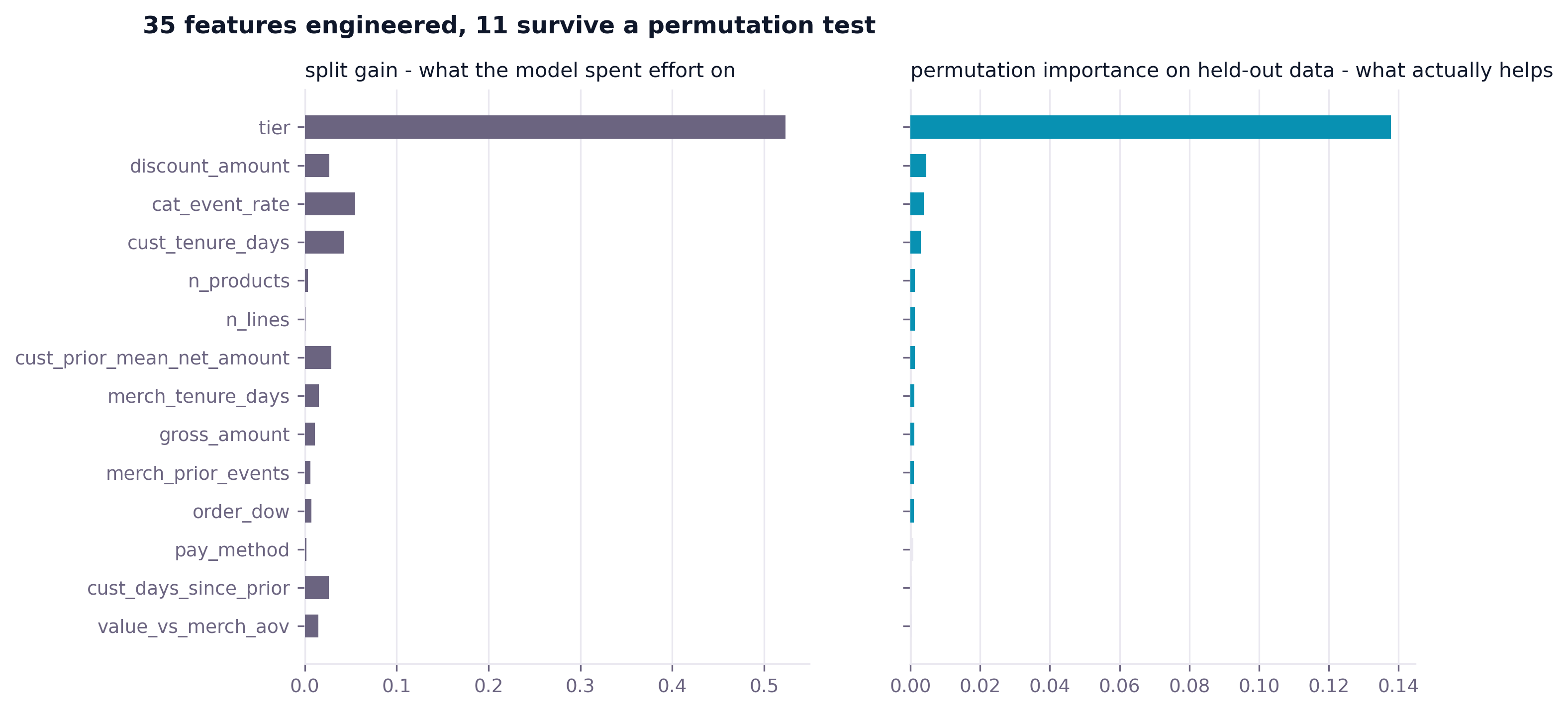
11 of 35 features clear a permutation test, but tier alone accounts for 92% of the total positive importance. The other ten are the tail of a noise distribution, which is exactly what a permutation test looks like when there is nothing left to find.

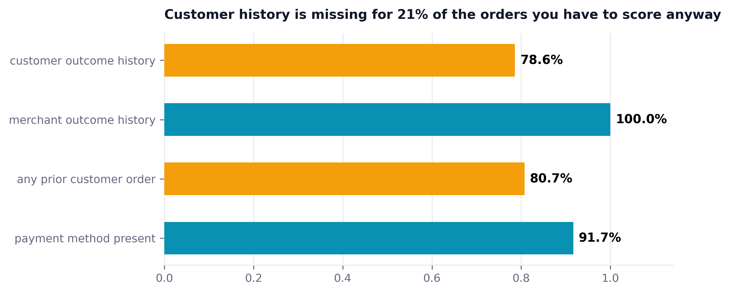
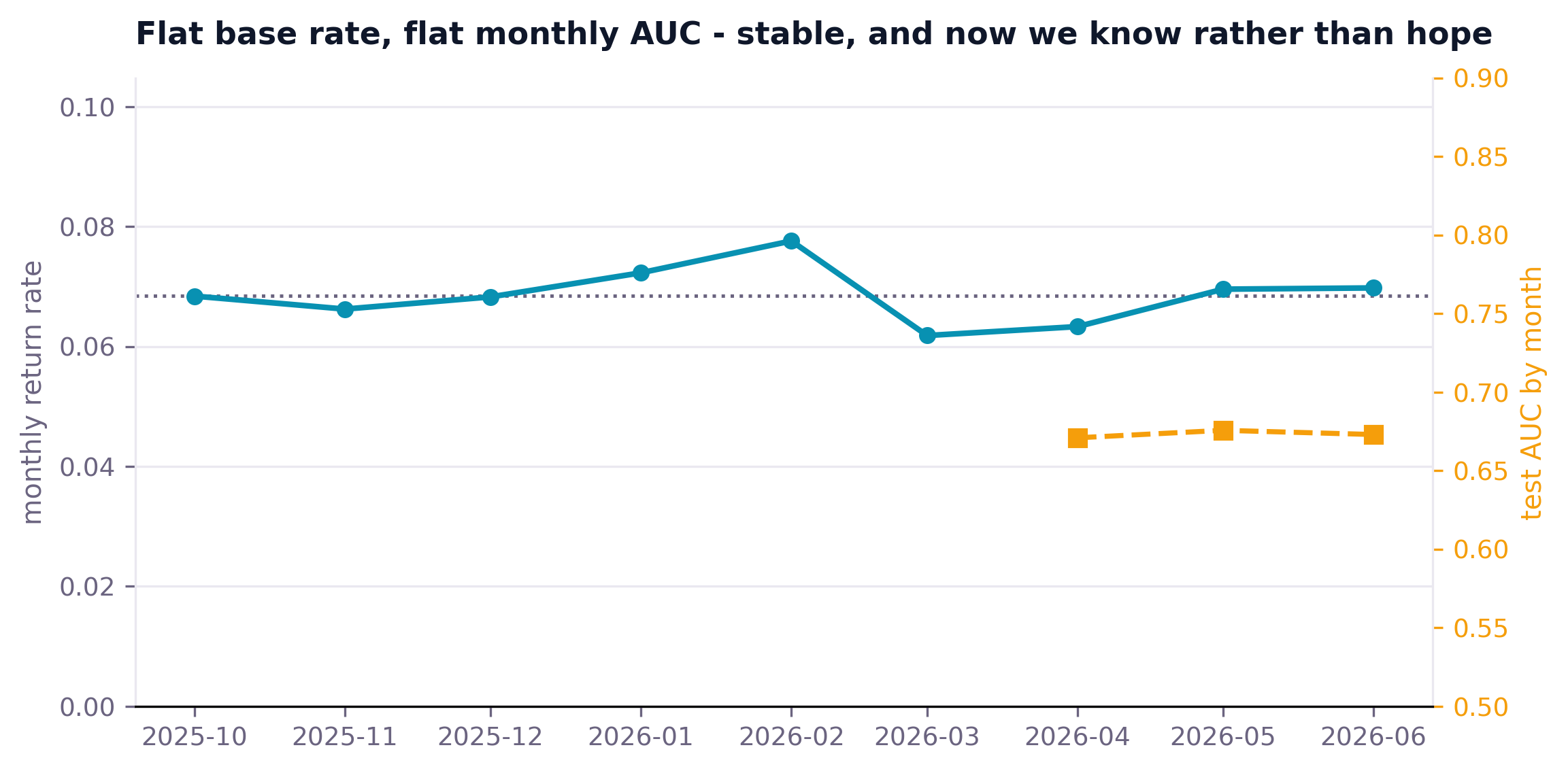
Left: roughly one order in five must be scored with the customer block missing entirely. Coverage is knowable on day one; check it before you invest in a feature family, because the fallback path is part of the model whether you designed it or not. Right: flat base rate, flat monthly AUC. The model is stable, and now that is known rather than hoped.

5g · The decision, in dollars

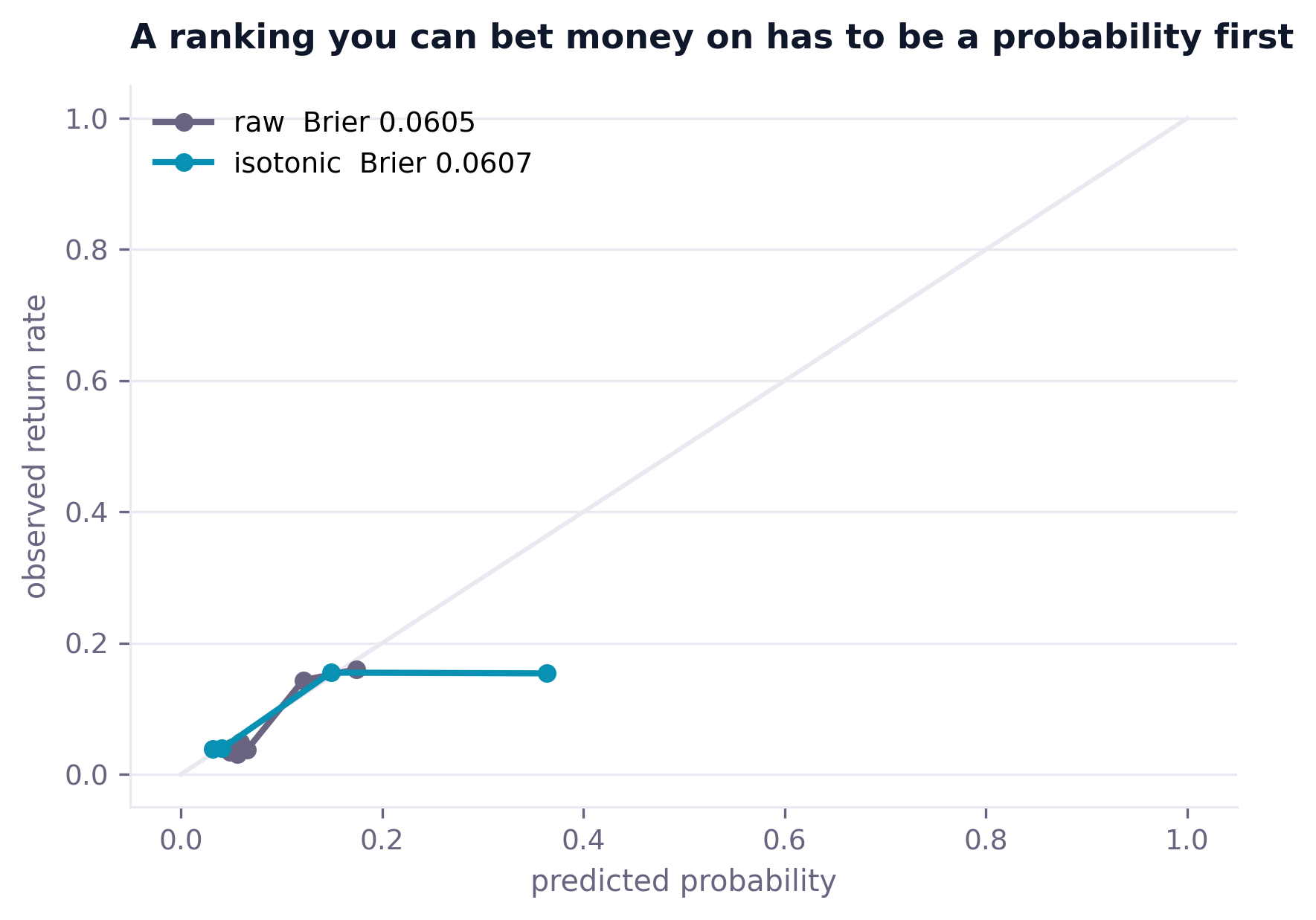
Calibration reported honestly: isotonic moved the Brier score from 0.0605 to 0.0607. It did not help. With so little real signal the model already produces near-calibrated probabilities at three levels, and fitting a calibration map on a small held-out slice adds more variance than it removes. Worth running, worth reporting either way.

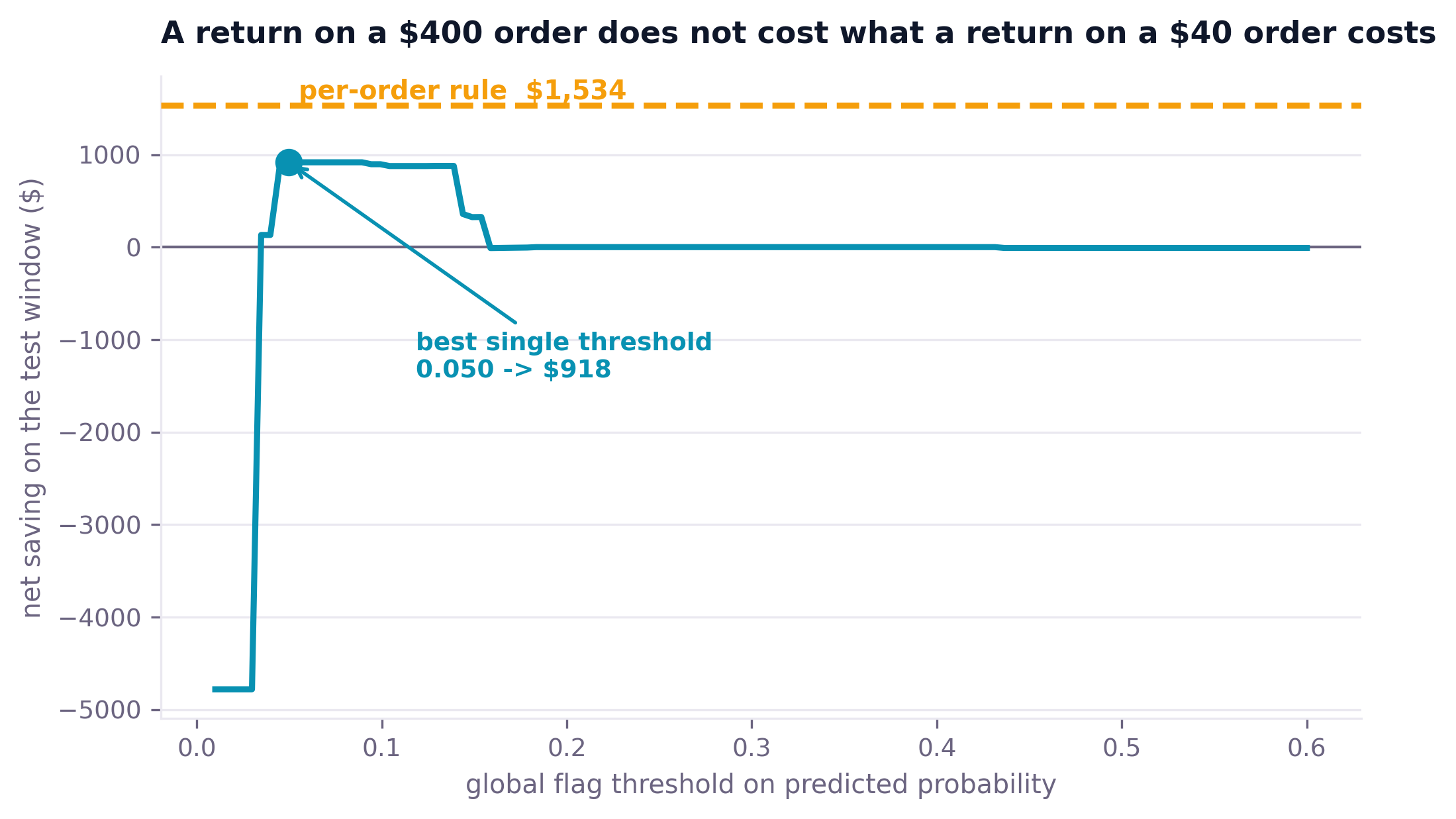
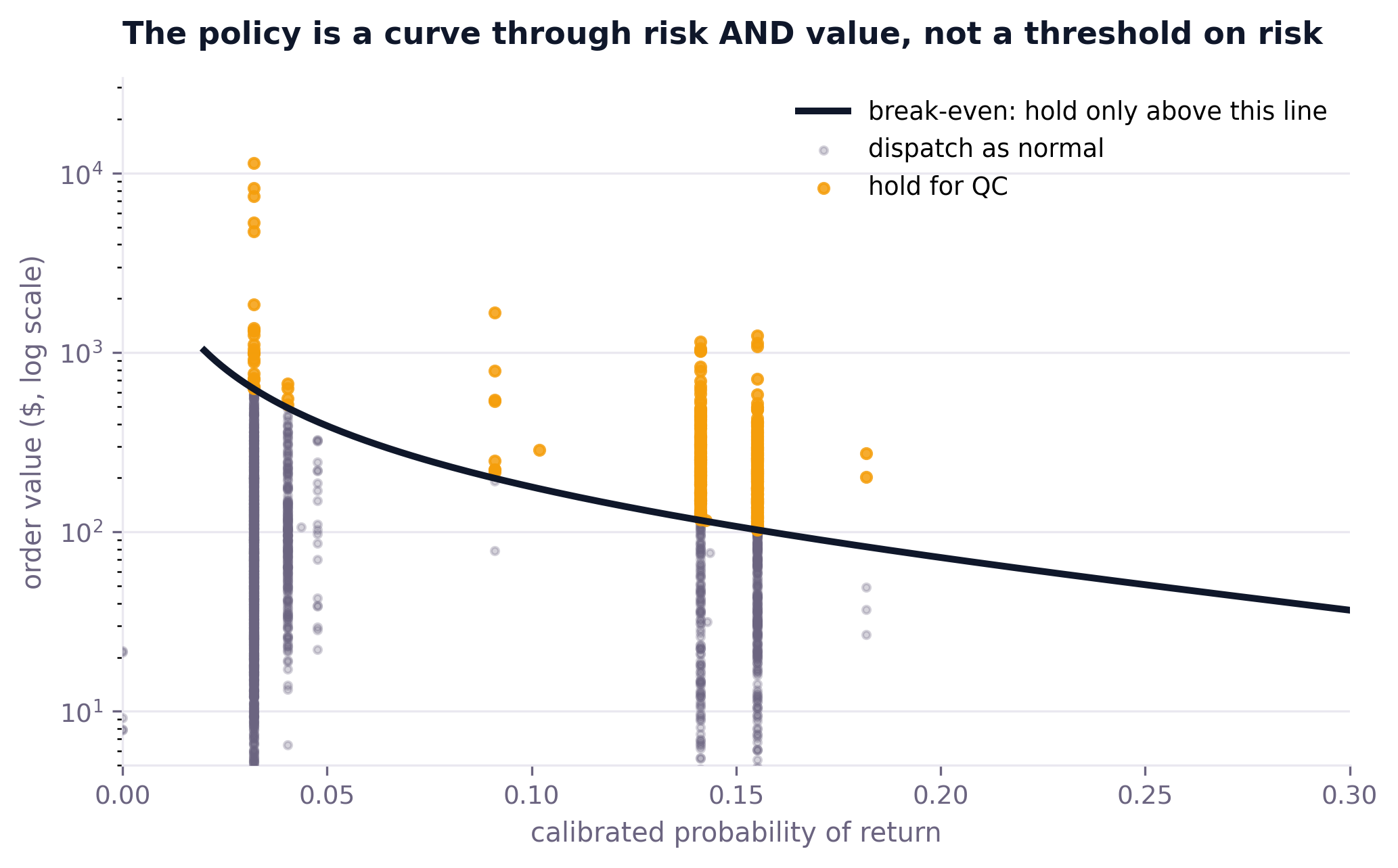
Act when p × effectiveness × cost_of_return > cost_of_hold. Because a return's cost scales with order value, that is a threshold per order, not one number - and it beats the best possible single cutoff by $600 on the test window. The policy is a curve through risk and value.

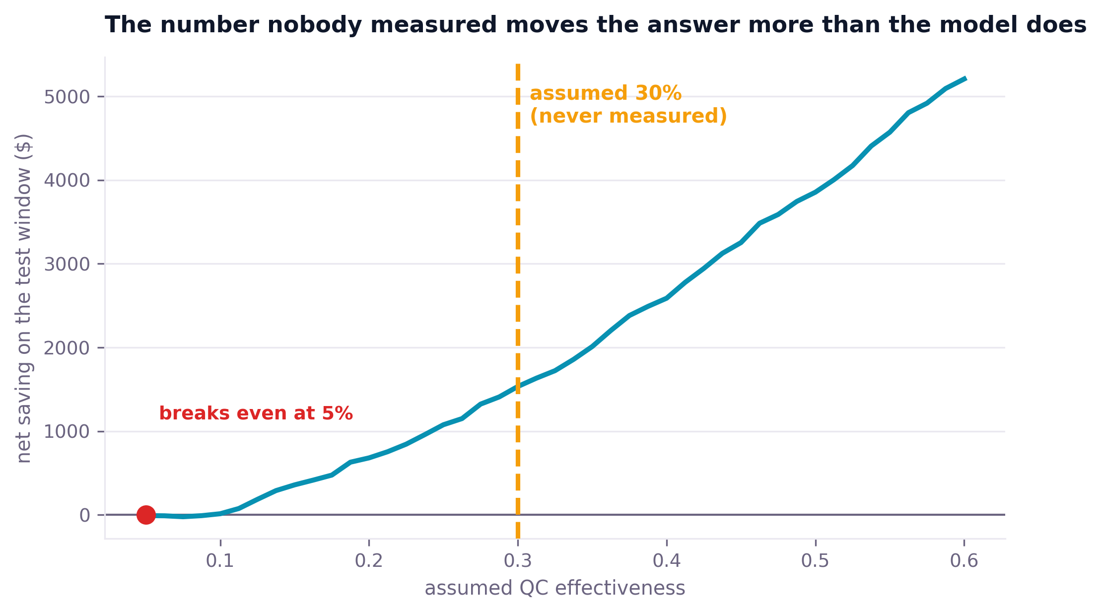
The declared assumption, swept. The programme breaks even near 5% against 30% assumed, so the policy has real headroom.

Two things are missing from that number, and both make it worse: the hold delays orders, and 85% of held orders were never going to come back - that customer cost is real and is not in the model. So the honest recommendation is not "ship the model". It is: run the hold manually on the 11.7% of orders the rule selects, measure effectiveness against a randomised holdout for one quarter, and revisit. If it comes back near 30% and volume grows, the engineering is a week. If it comes back near 5%, you have saved yourself the quarter.

5h · The scoreboard

Each rung is judged against the ceiling for its own population: a non-delivered order cannot be returned, so on the all-orders population the true probability is structurally zero there, which lifts the ceiling to 0.7486. Comparing every rung to one number would have been its own quiet error. Filtering M1 to delivered-only rows drops it to 0.6709 - the status leak disappears the moment the population matches what you will actually score.

Expert review - the panel that found a bug in the skill's own library

Five senior reviewer agents - ML methodology, data engineering, MLOps, commercial operations, executive insight - reviewed the v1 code and its real outputs. This was not polish. One finding was a genuine bug in a shipped module that had inflated a headline number by a factor of forty, and two findings changed what the page concludes. Every fix below is in the shipped code, and the whole pipeline was re-run afterwards.

# v1 (before): one comparison for every lag.
# At lag 0 this asks ts <= ts, so a row counts ITSELF, and its own label
# lands in its own "prior history" feature.
k = np.searchsorted(g_ts, g_ts - lag, side="right")

# v2 (after): strict when there is no lag, inclusive when there is
# strict at lag 0 so a row never counts itself or its timestamp twins;
# inclusive beyond that so a just-matured row is not thrown away
k = np.searchsorted(g_ts, g_ts - lag, side="left" if lag == 0 else "right")

# M3b: 0.9762 -> 0.6802. The leak the page was about to headline was ours.