how-to-sales-forecasting

Input - the marts, and the field that decides what counts as demand

This skill reads the marts produced by how-to-schema-and-warehouse. Two fields decide everything: orders.status (only delivered orders consumed stock) and orders.order_id - because if that key is not unique, every join fans out and the "demand" is partly fiction. It was not unique.

Sample data - the same seeded marts, and the traps a forecast walks into

No new generator: the marts already exist (seed 42). What matters is what is hiding in them - each trap planted on purpose, each one caught (or honestly declared unmeasurable) in Step 5.

Objective - a buy that survives finance, not a model that wins a leaderboard

Everrest runs consignment fulfilment: the platform commits inventory in advance. Committing low burns margin; committing high burns cash in holding and markdown. The question is never "which model has the best MAPE".

Find-skills - the forecasting toolbox

A demand plan needs a series layer, candidate models, a validation harness that cannot peek, and the economics that turn a distribution into a signable number.

Build - gate, measure, declare, then cost the decision

One deterministic script (seeded per random purpose - two runs are byte-identical) walks from raw marts to a buy paper. Grab the real code:

5a · The data-quality gate runs before anything is measured

The single most valuable "forecasting" step touched no model. 600 duplicate order rows - a retry bug, all in March - fan out against order_items and manufacture a whole phantom month.

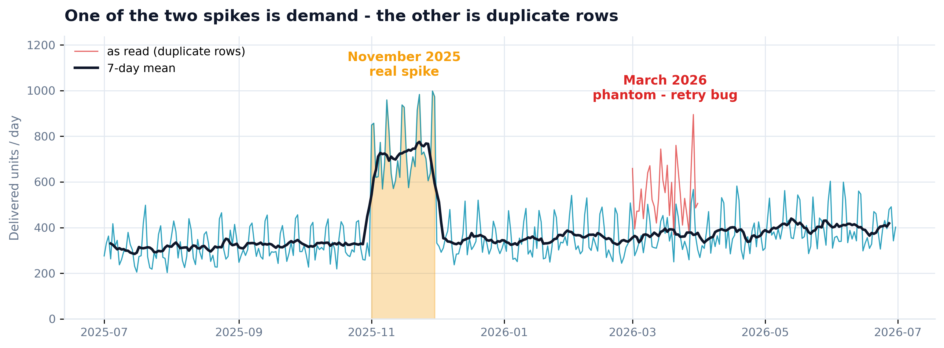
One year, two spikes - and only one survives the gate. The red trace is what the marts say as read; the cyan series is demand after deduplication.

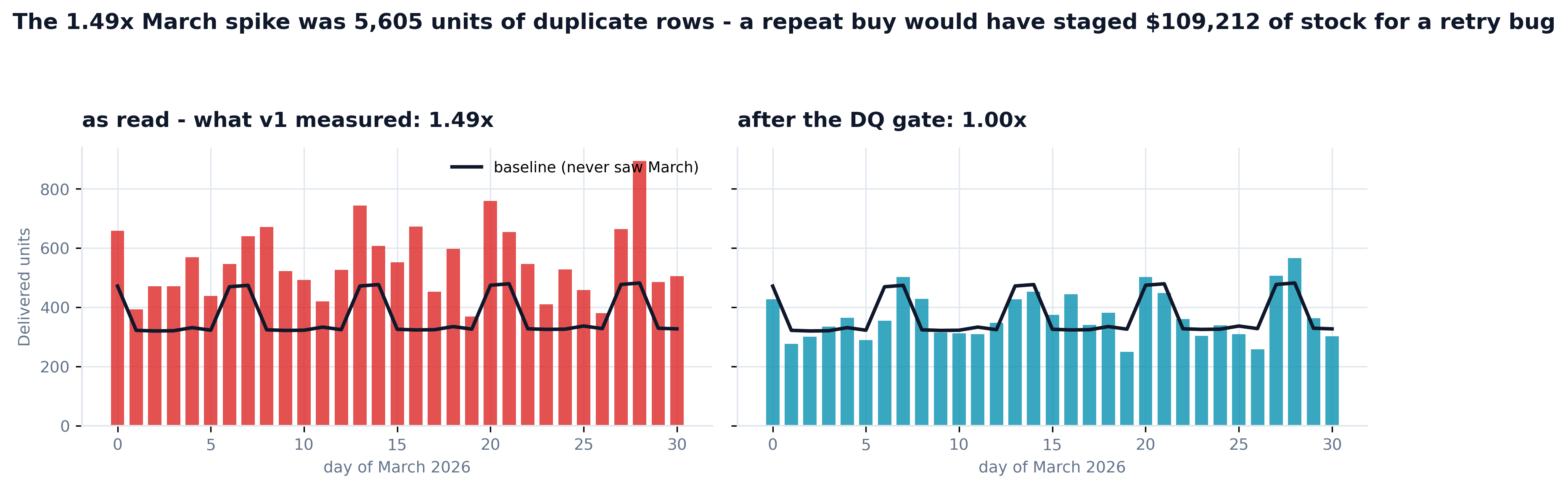
Same month, same baseline, before and after the gate: 1.49x becomes 1.00x. The v1 draft of this analysis skipped the gate, measured the phantom, and priced a repeat buy at $109,212 - the March recommendation is an engineering ticket, not a purchase order.

5b · Count the evidence before trusting any seasonality

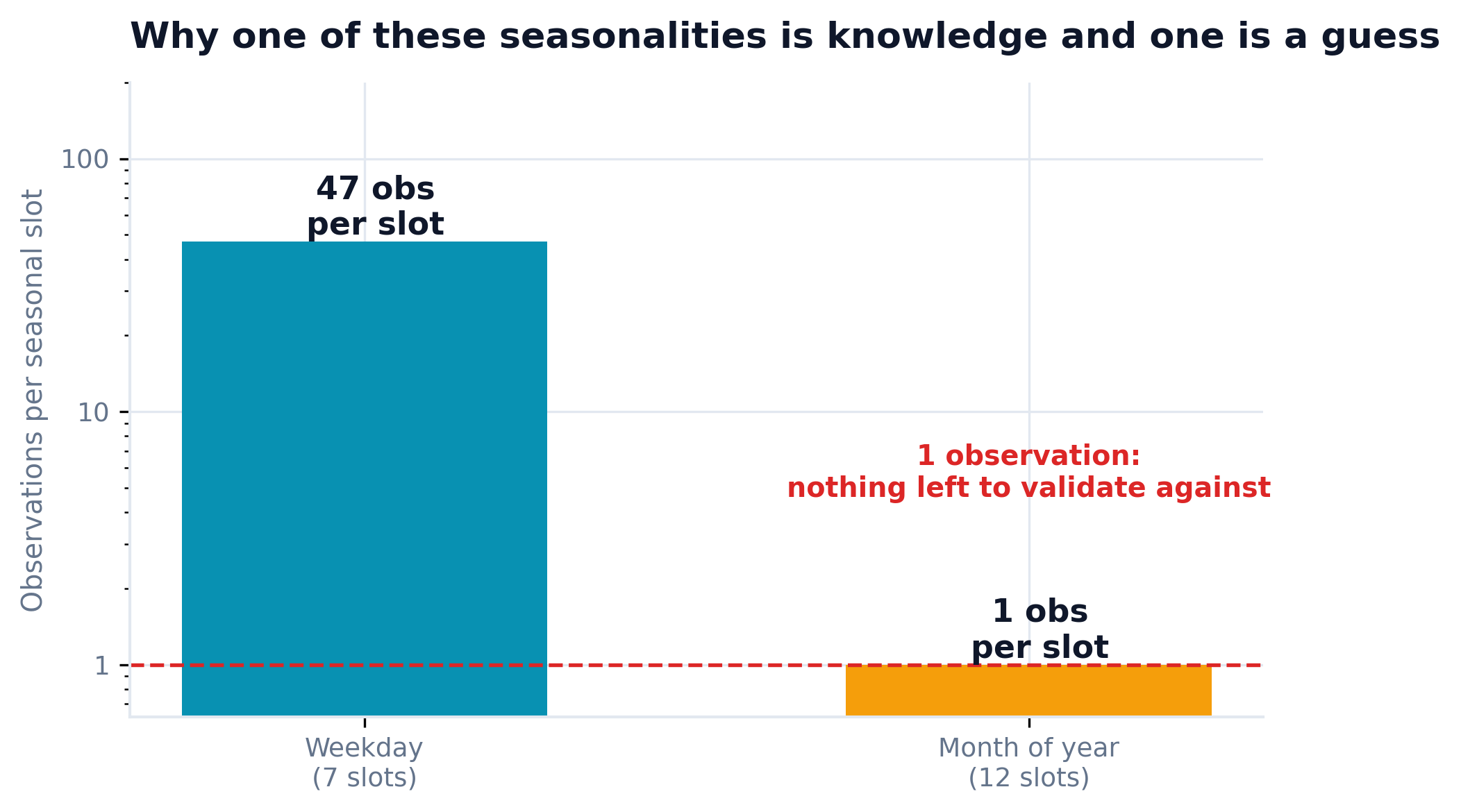
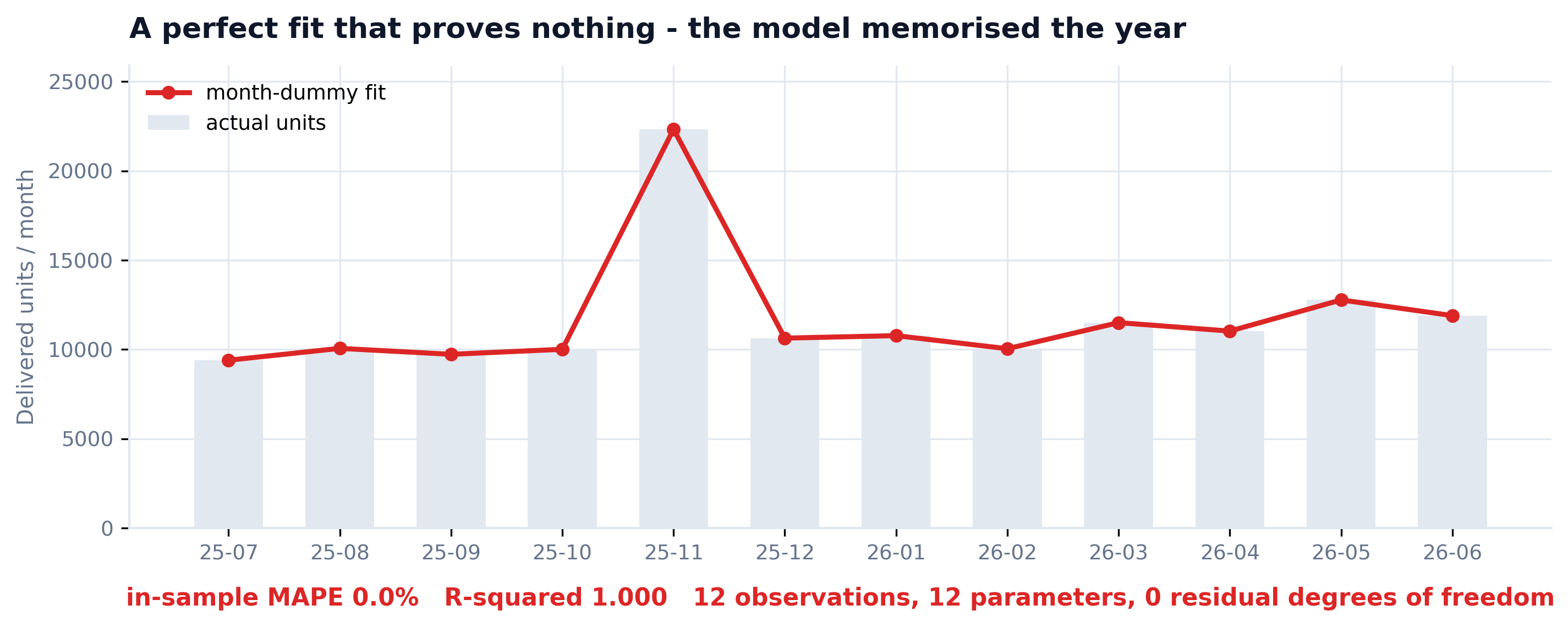
Left: weekday seasonality has 47+ observations per slot - knowledge. Month-of-year has exactly one - a guess. Right: the trap most tutorials fall into, shown rather than named: month dummies fit 12 points with 12 parameters, R-squared 1.000, and prove nothing.

5c · Two backtests, two honest winners

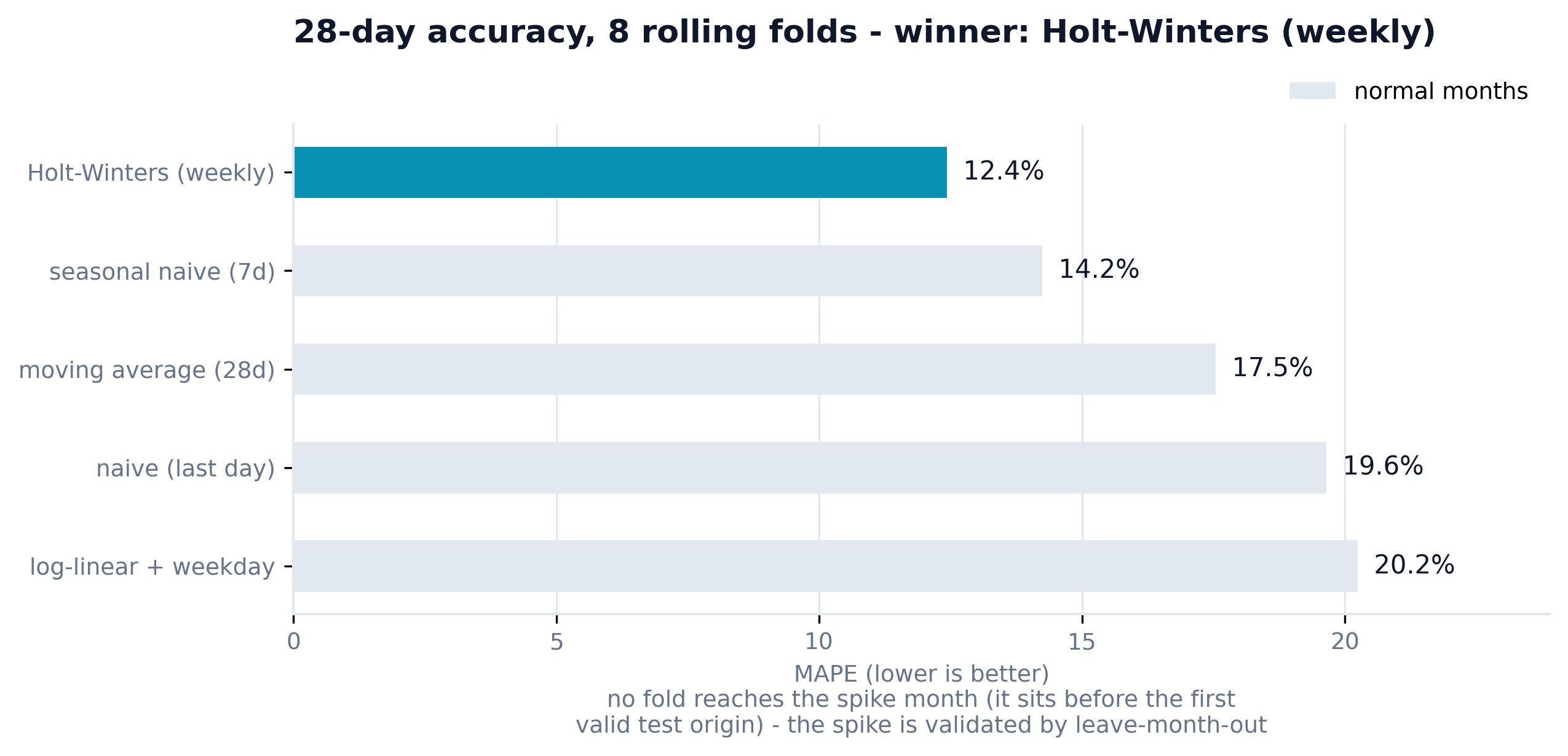
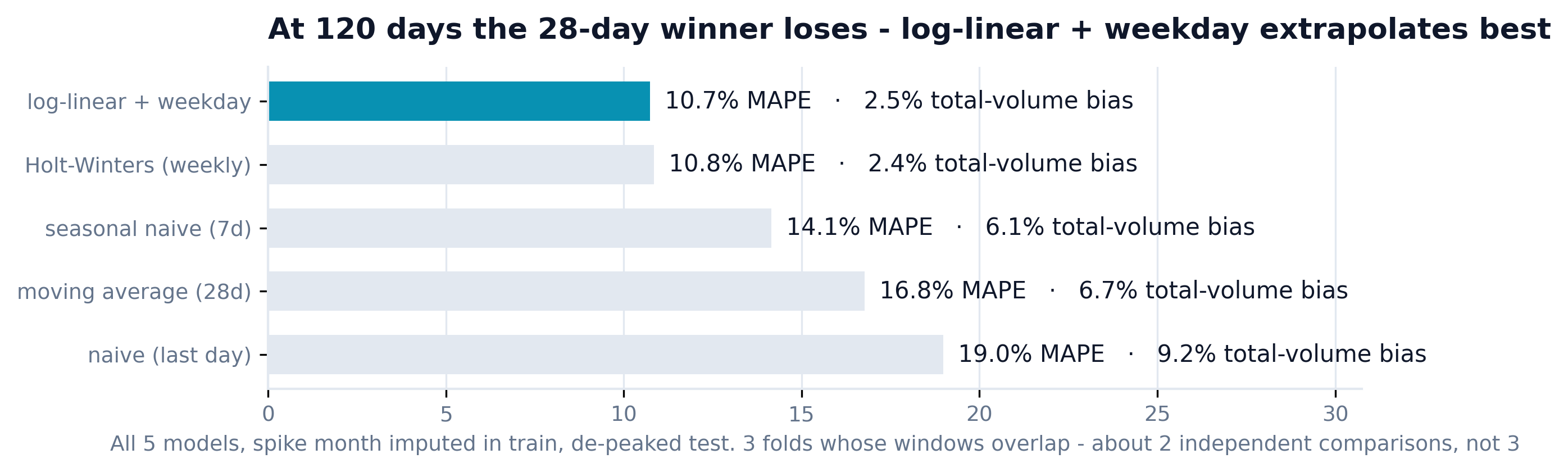
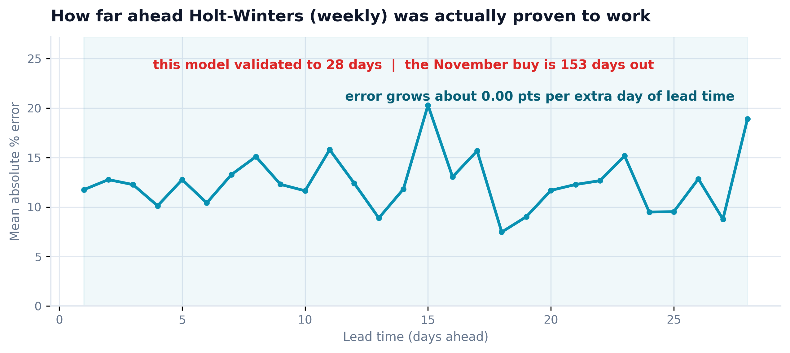
Left: at 28 days Holt-Winters wins (12.4% MAPE, 8 rolling folds). Right: at the 120-day planning distance the ranking flips - all five models race on a spike-imputed series, and log-linear + weekday takes it by a nose (10.7% vs 10.8%). The chart also confesses its own weakness: 3 overlapping folds are about 2 independent comparisons. The buy is 153 days out - past the last validated point, and the memo says so.

5d · Size the one real spike against a baseline that never saw it

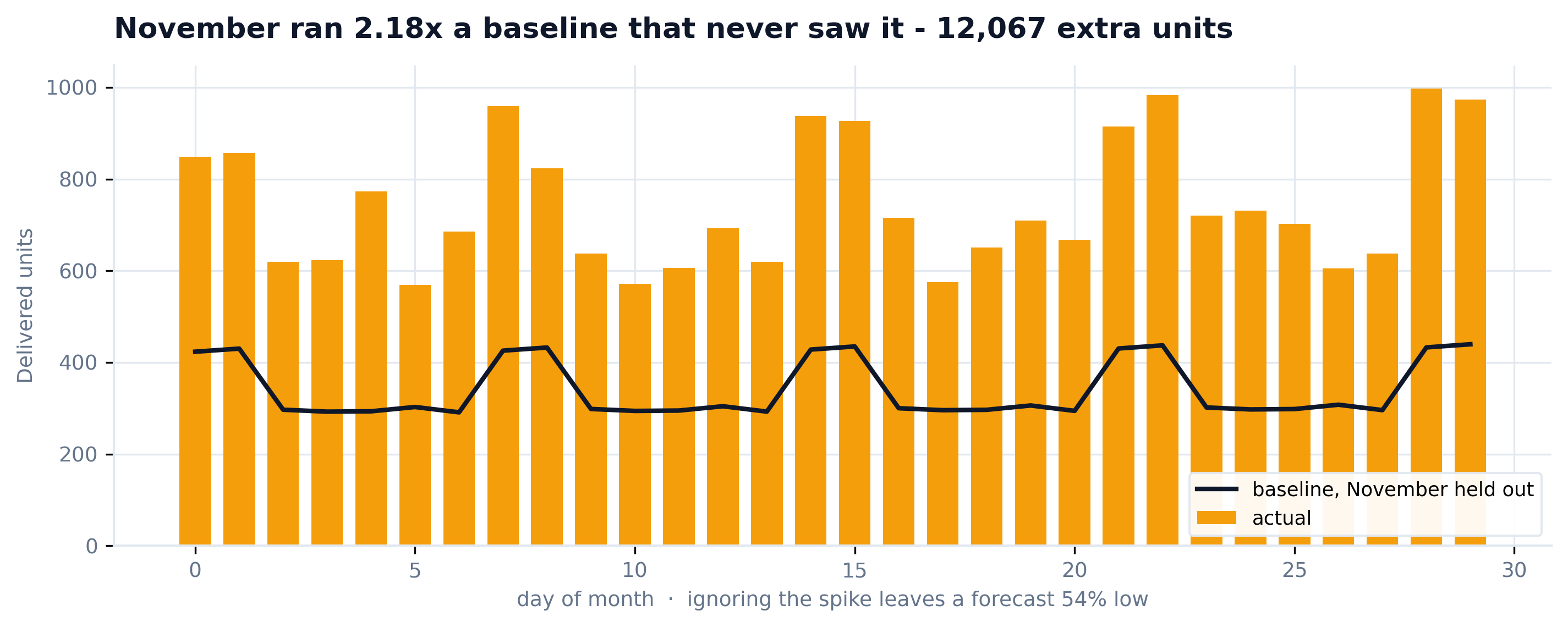
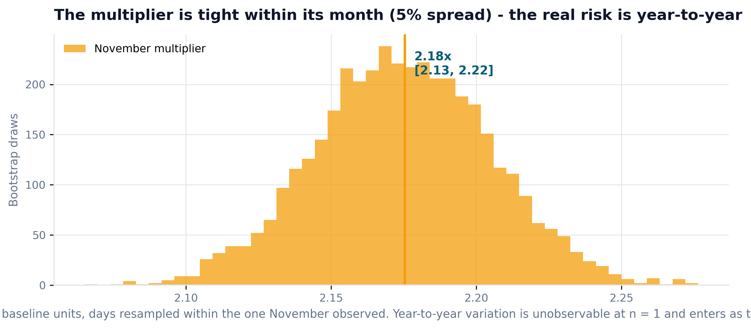
Left: November ran 2.18x a baseline fitted with the spike held out - 12,067 extra units. Right: the multiplier is tight within its month (5% spread). The dangerous uncertainty is year-to-year - unobservable at n = 1 - so it enters as a declared sigma with a sensitivity chart, never as a fake confidence interval.

5e · Turn the distribution into a signable buy

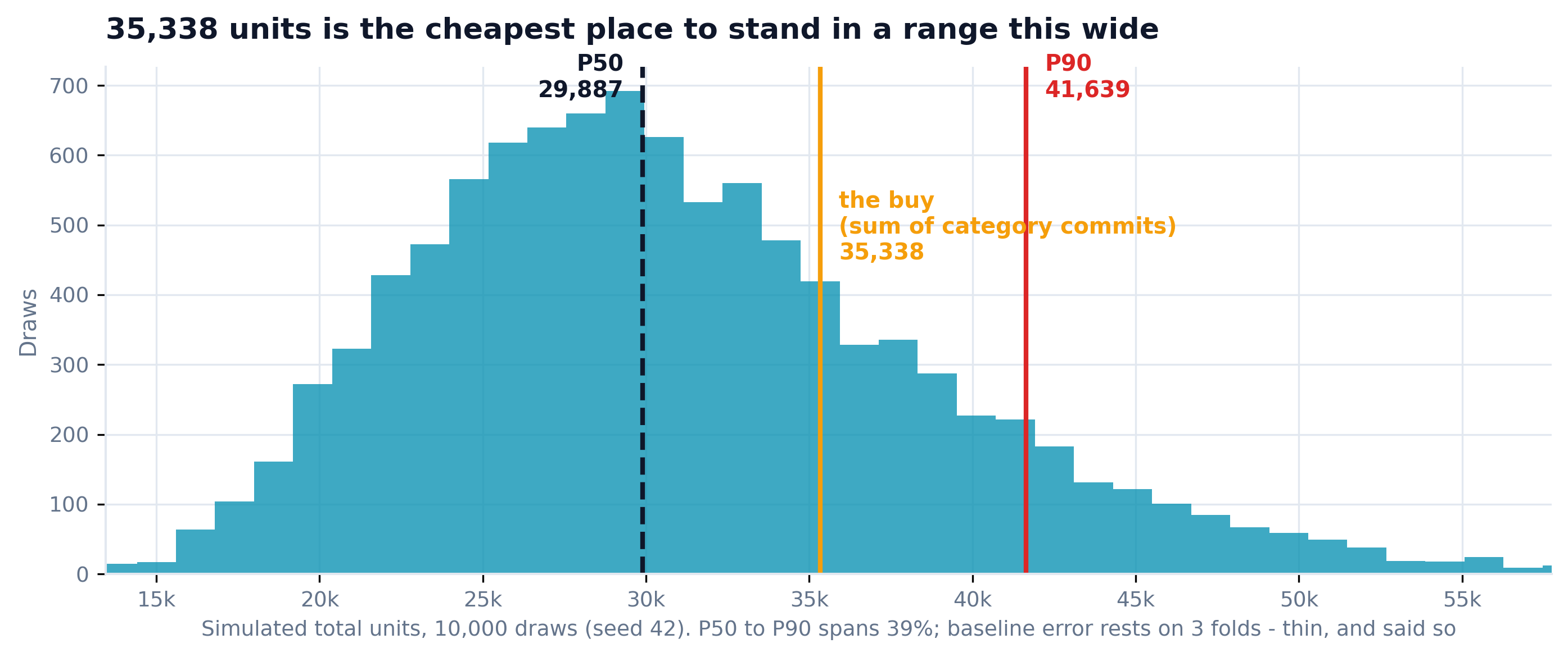
10,000 seeded draws: measured baseline error x measured day variation x the declared year sigma. The buy stands at the newsvendor optimum - above the middle, because being short costs 20% of price and being long costs 8%.

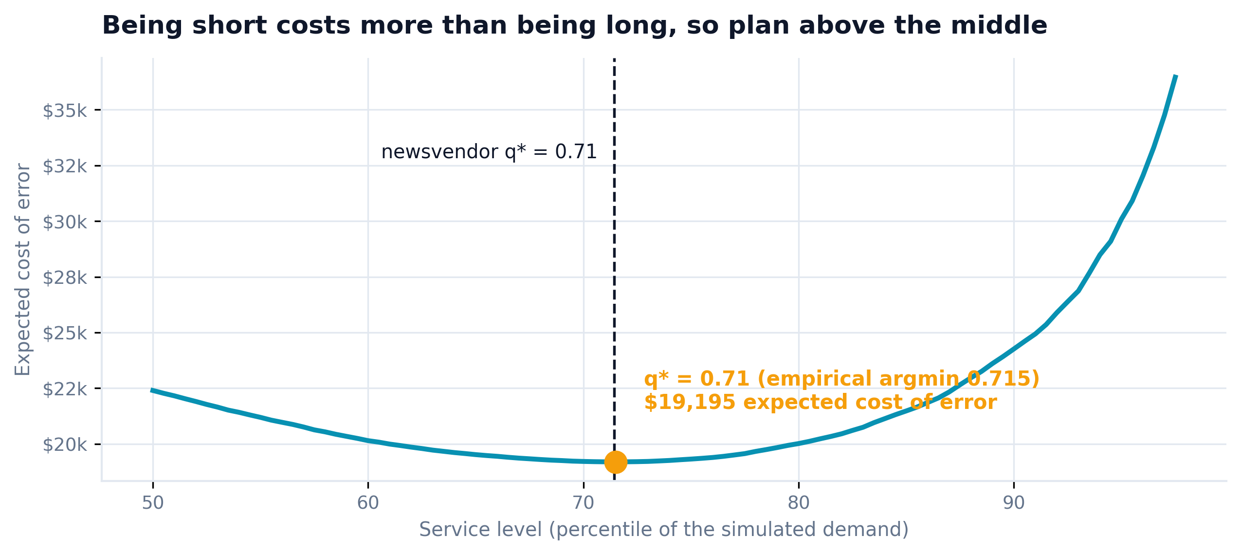
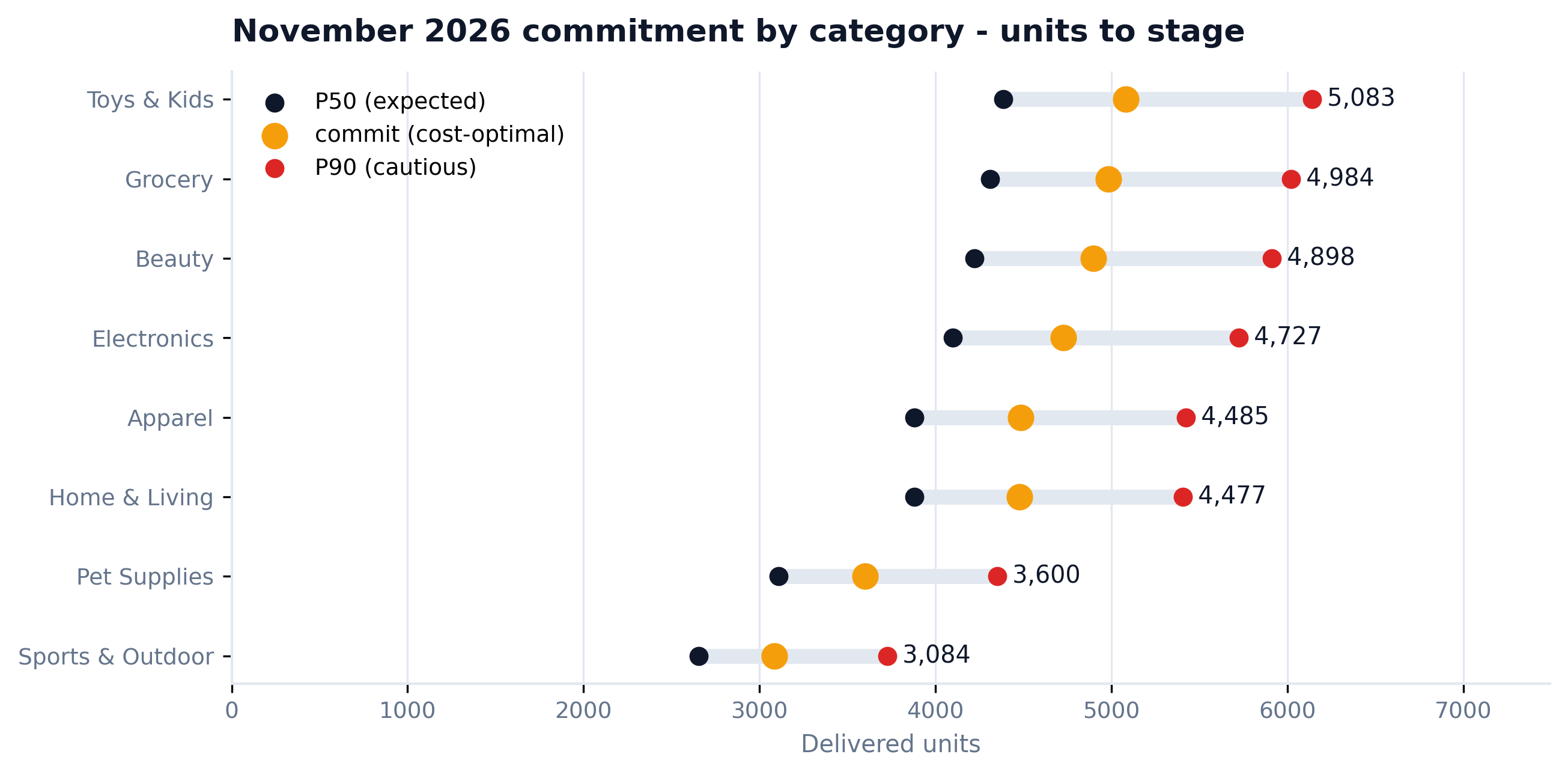
Left: the analytic q* (0.71) lands on the empirical cost minimum - the model checks itself. Right: every category simulated on its own baseline and its own multiplier - a real per-category newsvendor, not one pooled quantile split by share.

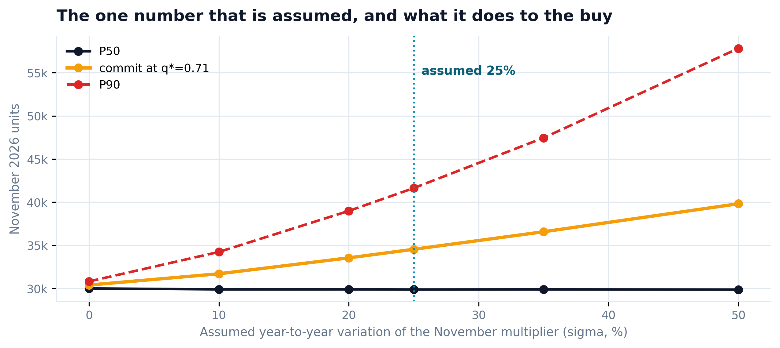
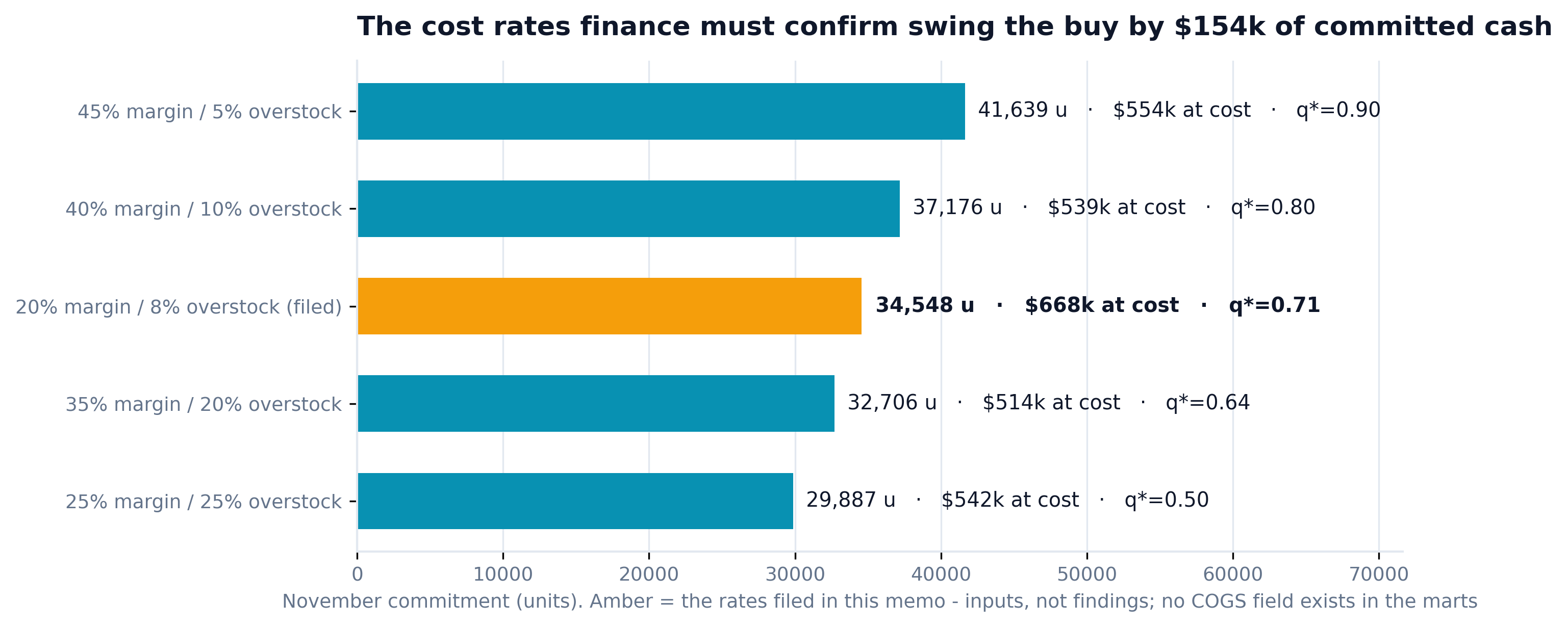
Left: the ONE declared unknown, swept: the commit moves 31% across sigma 0-50%; the P90 nearly doubles its distance. Right: the sweep most forecasts never run - the margin/overstock assumption swings the buy by $154k of committed cash, as hard as the model itself. Both are inputs; both get charts.

Expert review - the panel that found a phantom, a sign error, and a fake trend

Five senior reviewer agents - forecasting methodology, supply-chain planning, executive insight, data engineering, commercial P&L - reviewed the v1 code and its real outputs. This was not polish: three findings changed the numbers, one changed the story. Every fix below is in the shipped code.

# v1 (before): agg_rel_pct = (pred - actual) / actual, so truth = pred / (1+e).
# Multiplying applies the model's bias in the WRONG direction:
base = baseline_total * (1 + RNG.choice(long_resid, size=n))   # shifts LOW
yoy  = np.exp(RNG.normal(0, sigma, n) - sigma**2 / 2)          # mean-preserving, median sags

# v2 (after): divide to invert, drop the sigma^2/2 so the MEDIAN stays put
base = baseline_total / (1.0 + resid_draws)                    # under-forecast bias corrected UP
yoy  = np.exp(z * sigma)                                       # median 1.0 at every sigma